Article
Current Flows,
Current probes,
3D Field Solver,
Impedance,
Return path
A Simple Demonstration of Where Return Current Flows
For ten years, I’ve had the honor of presenting a tutorial session at the IEEE EMC Symposium. I’m usually positioned right after Bruce Archambeault. This means I get to listen to Bruce talk about inductance. While I think of myself as a bit of an expert on inductance, I always learn something new when I listen to Bruce.
One example he shows, using a simulation of where current flows, will completely recalibrate your intuition if you have never thought about this question. This example stuck with me for more than a dozen years since I originally saw it. Recently, I had a chance to play with the Teledyne LeCroy CP031A current probe used with our scopes and I realized this classic simulation example could be demonstrated with a simple measurement.
Simulating Where Return Current Flows
Bruce published his simulation in the IEEE EMC Magazine in 2008. Using his IBM proprietary 3D field solver, he built a U shaped microstrip with a signal launched into one end, terminated to the plane at the other end. He sent in a sine wave at 1 kHz and plotted the current in the signal conductor and the return current distribution in the plane. Then he changed the frequency to 50 kHz and then 1 MHz. The return current distribution in the plane below the signal trace dramatically changes. Figure 1 shows his simulated result for these three different frequencies.
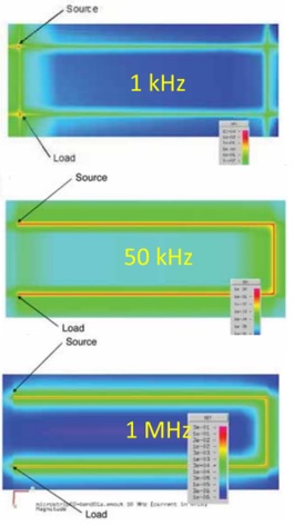
Figure 1. Bruce Archambeault’s simulation of the signal and return current in a microstrip. This is the result from a proprietary IBM field solver. Reprinted with permission.
At low frequency, all the return current takes the shortcut across the plane between the two ends of the signal trace. But at frequencies above 1 MHz, there is no return current between the ends of the microstrip. It all travels directly underneath the signal path.
Why does the return current take the long path all the way around underneath the microstrip instead of the short path between the two ends? It’s all about impedance. The return current path is always going to take the path of lowest impedance.
The impedance at any frequency is related to 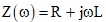
At low frequency, the impedance is all about the resistance, the shortest length, directly across the plane. At higher frequency the jwL term begins to dominate, and the current redistributes to take the path of lowest loop inductance.
Of all the different paths the current can take, the path of lowest loop inductance is when the return current path is as close, underneath the signal current as it can get. The current redistributed to be directly underneath the signal path to minimize the loop inductance.
In Bruce’s simulation, the redistribution begins between 1 kHz and 50 kHz and is complete by 1 MHz. For all currents on a circuit board above 1 MHz, the return current is always flowing directly underneath the signal path. This is one of the most important principles in SI, PI and EMI.
Can We Measure the Path the Return Current Takes?
Todd Hubing shows a similar example from a measurement in his lab of the amount of current flowing through a ground strap between the ends of a coax cable, reproduced in Figure 2.
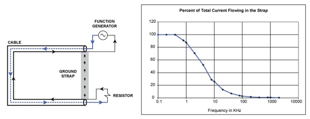
Figure 2. Example of the measured return current distribution in a short connection between the ends of a coax cable. Reprinted with permission.
As soon as I got my CP031 a current probe, I realized I could reproduce Todd’s experiment very quickly and easily with a simple set up.
A clamp-on current probe is a specialized scope probe which clamps over and encircles a wire. The probe measures the current that flows through the wire passing through the center hole. It does this by using an iron core making up an annulus around the wire, with a small gap at the clamp. The high permeability of the iron amplifies the magnetic field from the current in the wire. It is concentrated in the small gap.
A Hall Effect magnetic field sensor sits between the pole faces where the magnetic field is highest. The sensor’s output voltage is related to the magnetic field which is related to the current in the wire inside the clamp. One of the key advantages of this probe is that it is sensitive to DC currents, as well as high frequency.
The bandwidth is limited by the frequency dependence of the permeability of the iron and the bandwidth of the amplifier. The bandwidth of the CP031A is 200 MHz. The clamp-on current probes come from the factory already calibrated in mA. They communicate to the scope over a Pro Bus, a smart sensor bus, that allows the scope to read the calibration information and display mA on the front screen.
I took a common RG174 50 Ohm coax cable with BNC connectors on the ends and soldered a shorting wire between the two ends of the coax shield. This is shown in closeup in Figure 3.
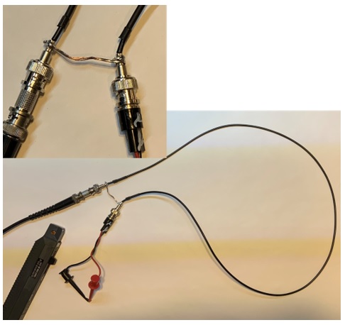
Figure 3. A coax cable with the ends of the shields connected with a grounding strap, shown in closeup.
I used a LeCroy WaveStation 2052 50 MHz Waveform generator to create a swept sine wave of current. The way to make a constant current AC source is to use a constant voltage sine wave source, with a 50 Ohm source resistance and just short the ends.
I set up the function generator for a 3 V peak to peak sine wave into a 50 ohm load. This means the internal voltage source was 6 V peak to peak. When the output is shorted, the 6 V source is across the 50 ohm output resistance, is a current of 6 V pk-pk/50 ohms = 120 mV pk-pk. I used the CP031A current probe to measure the current through the shorted ends of the coax cable, as shown in Figure 4. I measured a 10 kHz sine wave of current with a 120 mA pk-pk value, just as expected.
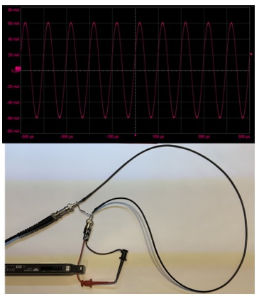
Figure 4. Top is the measured current through the signal wire in the coax cable with a 10 kHz sine wave from the function generator.
The function generator drives this 120 mA pk-pk current through the coax cable. I swept the frequency from 1 kHz to 5 MHz with a sweep time of 1 minute.
At the end of the cable, I separated the signal and return conductors with a mini grabber so I could measure the current through the signal conductor with the CP031A current probe. It should be flat in frequency if the function generator produces a constant voltage amplitude. By measuring the current through the signal lead of the minigrabber, we get an idea of the flatness of the current amplitude over the frequency range.
As the frequency of the sine wave increased, I measured the current waveform with a Teledyne LeCroy WavePro HD scope, with an 8 GHz bandwidth and 12-bit vertical resolution. The setup is shown in Figure 5.
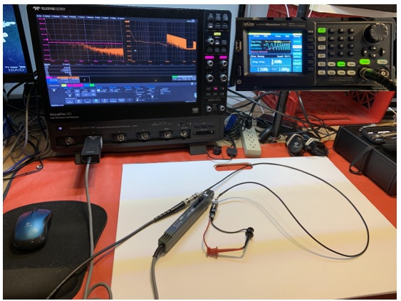
Figure 5. The WavePro HD scope, WaveStation function generator and the modified coax cable with CP031A current probe.
Measuring the Return Current in the Shunt Over Frequency
As the sine wave of current changed frequency, the FFT was constantly calculated and the peak hold setting was used to record the maximum recorded amplitude of the current. As the current swept through its range, the peak hold setting captured the peak amplitude across the spectrum. This is a simple way of implementing a transfer function plot if your scope does not have a tracking function generator. Figure 6 shows the recording of the amplitude distribution of the current through the signal path as the frequency swept.
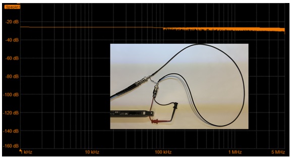
Figure 6. The measured frequency response of the current through the signal conductor is very flat from 1 kHz to 5 MHz. Vertical scale is the current amplitude in dB and horizontal scale is the frequency of the FFT calculation, on a log-log scale.
This shows a very flat current response through the signal path. This is a combination of the constant amplitude of the current source, the response of the current through the signal path and the bandwidth of the CP031A current probe. This flat response is exactly what we would expect.
Normally in a coax cable the signal current travels on the central conductor and the return current travels in the outer shield. But, when I shorted the two ends of the shield together, the return current had a chance to take a shortcut by jumping from one end to the other through the shunt.
At DC, the return current flows from the front end of the shield to the back end of the shield through the shorting shunt. Using the current probe, we can literally measure the current flowing through the shortcut at any frequency. The measurement is shown in Figure 7.
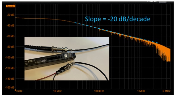
Figure 7. The measured frequency response of the current amplitude through the shorting shunt between the two ends of the coax return path. A line with slope of -20 dB/decade is superimposed.
In this measurement, the current through the shortcut shunt starts out with all the current flowing through the shunt at low frequency below 10 kHz. It begins to drop off at about 10 kHz. Above 10 kHz, the current amplitude through the shunt drops off like 1/f. This is reasonable since the impedance of the inductance increases ~ f and the current should redistribute into the alternative path of lower loop inductance inversely with the impedance.
This measurement indicates that above 10 kHz, the return current in this specific geometry will begin to redistribute to take not the shortest path, but the lowest loop inductance path. In this geometry, the path of lowest loop inductance is when the loop area between the signal and return paths is a minimum which is when the signal and return current paths are as close together as possible.
Since the signal current is confined to the central signal conductor, this means the return current will flow coaxially around the signal current all along the coax, and not shunt between the beginning and ending of the shields.
At 1 MHz, there is only 1% (40 dB down from the 1 kHz value) of the current amplitude taking the shortcut thru the shunt conductor compared to at 1 kHz, and it continually decreases to smaller values with every higher frequency.
The Time Domain View
The plot of the amplitude of the current through the shunt as a function of frequency is basically a Bode plot. This behavior is a 1-pole low pass filter. This behavior makes it easy to anticipate the transient response.
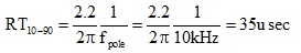
If we send a step current of 120 mA of current through this modified coax cable, the current taking the shortcut through the shunt will be a low pass filtered version of the step. It will have a 1-pole response just like an RC circuit. The pole frequency, where the response has decreased by -3 dB, is about 10 kHz. The expected 10%-90% rise time of the current through the shunt with a pole frequency of 10 kHz is:
I used a 120 mA peak-to-peak square wave of current from the WaveSource, with a rise time of about 15 nsec. This was sent through the coax and was measured with a second current probe at the far end of the coax.
The high frequency components of the return current should not pass through the shunt, only the low frequency. In fact, we should see a rise time of about 35 usec for the current to turn on through the shunt. Figure 8 shows the step response of the current through the coax and the slow rise in the current through the shunt. The measured 10-90 rise time is 32 usec, very close to what we expected.
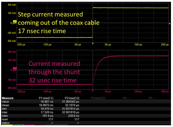
Figure 8. The step response of the current through the coax.
In a microstrip transmission line with a return plane under the signal paths, the return current will change its path depending on how quickly the current changes. If the rise times of your signals are on the order of 10 usec or longer, which is in the audio range, the return current in the plane will spread out and take the path of lowest resistance. But, if the rise times of your signals are shorter than 10 usec, the fast edge current will all travel directly underneath the signal lines.
Conclusion
This simple measurement demonstrates the most important principle in SI/PI and EMI, that the return current will flow in the path of lowest resistance below about 10 kHz. But above about 10 kHz, the return current will begin to redistribute in the return path to be adjacent to the signal conductor. In this specific geometry, by 1 MHz, 99% of the return current is flowing adjacent to the signal conductor. The precise frequency where most of the return current is flowing adjacent to the signal path will vary depending on the specific geometry, but this is a good rule of thumb to keep in mind.
Even though alternative current paths are provided, the current will not take these paths but always take the path of lowest loop inductance. Like Mary’s little lamb, above 10 kHz, wherever the signal current goes, the return current is sure to follow.
-Eric Bogatin
Related Topics:
No Related Topics at this time.